Kitagawa Model

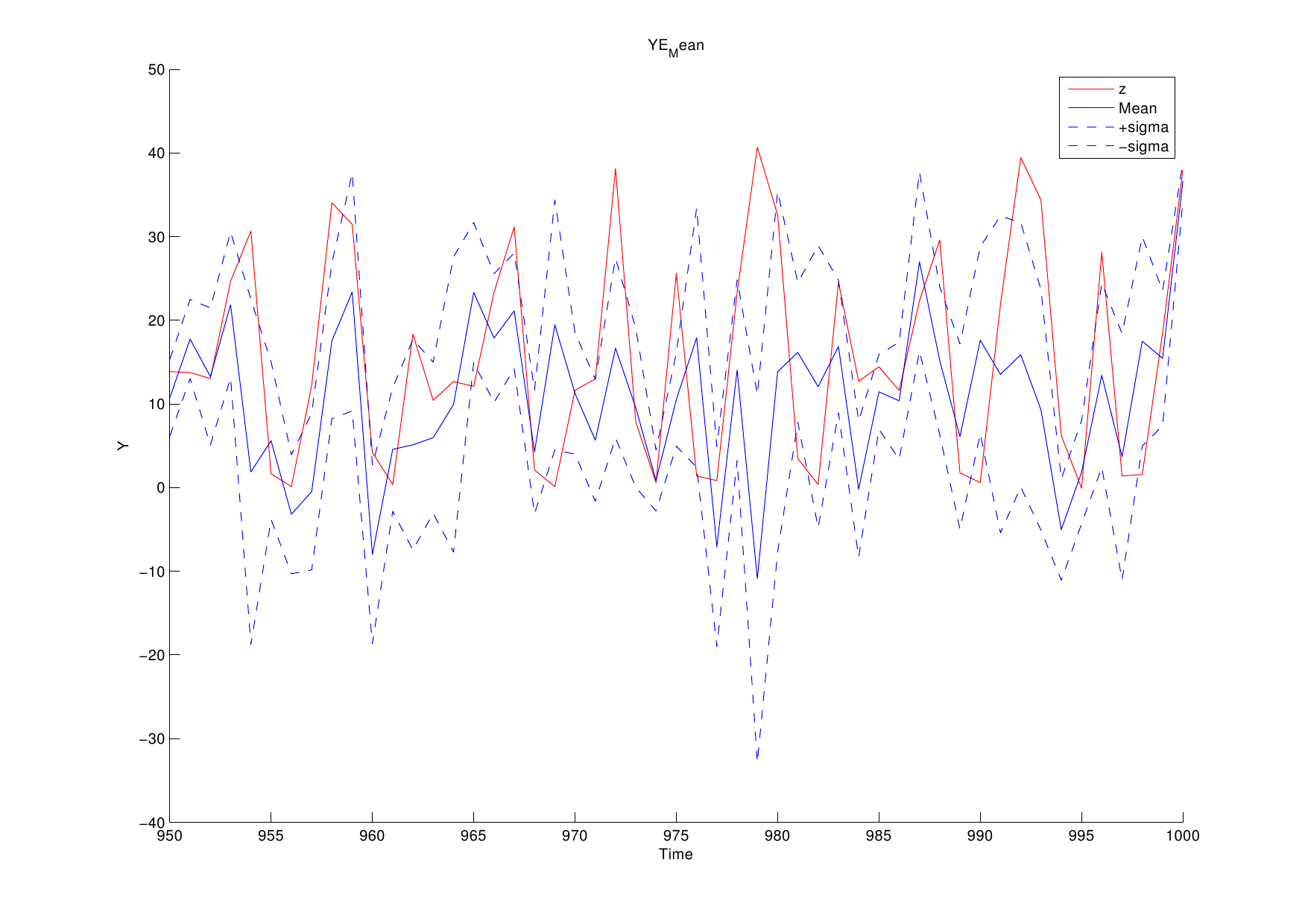
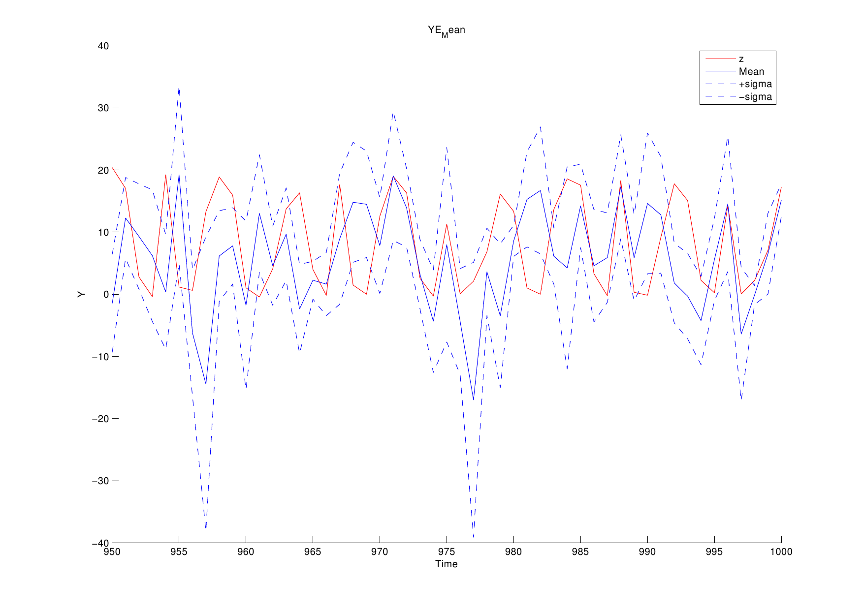
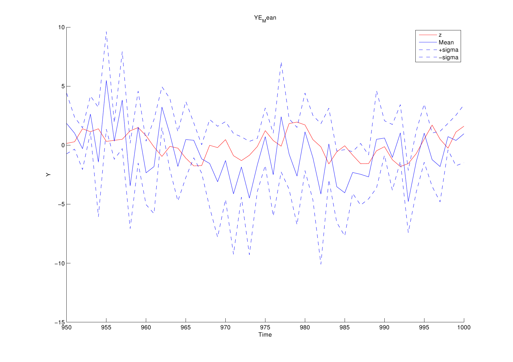
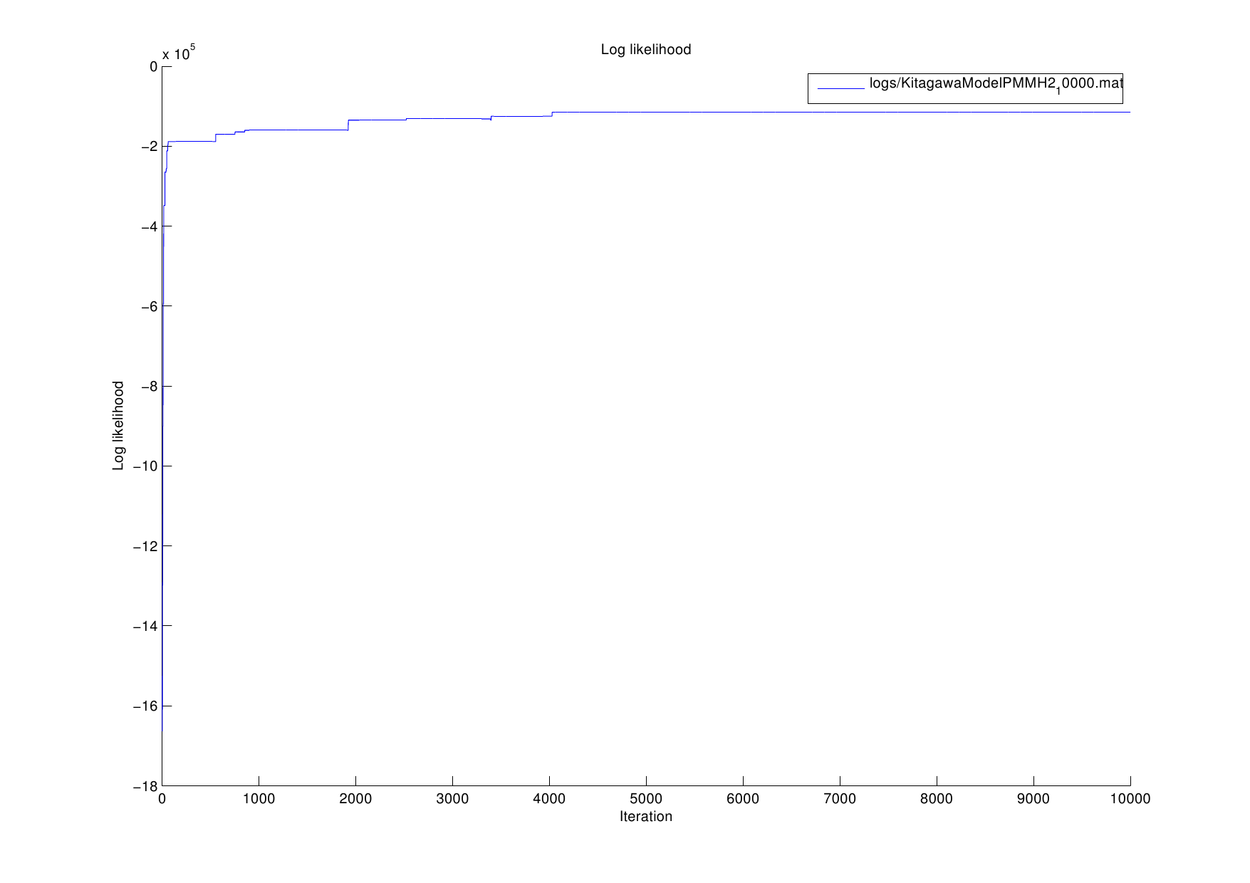
Here we introduce the example of model estimation using the MCDC tool, given observed sequences generated by the generalized Kitagawa model given by the following SSM:

State transition function:
x1(t) = a1 * x1(t-1) + b1 * x1(t-1) / (1 + x1(t-1) ^ 2) + c1 * cos(1.2 * t) + sqrt(q1) * randn;
x2(t) = a2 * x2(t-1) + b2 * x2(t-1) / (1 + x2(t-1) ^ 2) + c2 * cos(1.2 * t) + sqrt(q2) * randn;
Observation function:
y1(t) = d1 * x1(t) ^ 2 + d2 * x2(t) ^ 2 + sqrt(r1) * randn;
y2(t) = d3 * x1(t) ^ 2                  + sqrt(r2) * randn;
y3(t) =                  d4 * x2(t)     + sqrt(r3) * randn;

where a1, a2, b1, b2, c1, c2, d1, d2, d3, and d4 are the model static parameters. The parameters q1, q2, r1, r2, and r3 control the magnitude of state transition/observation noise.


Parameter setting for Kitagawa model
Parameter name
Description
Value
T length of data sequence 1,000
(a1, b1, c1) model parameters for state variable x1 (0.5, 28, 8)
(a2, b2, c2) model parameters for state variable x2 (0.6, 30, 10)
(d1, d2, d3, d4) model parameters for observation variable y
(0.05, 0.06, 0.07, 0.08)
(q1, q2) magnitude of noise added to state transition function
(1e-1, 1e-1)
(r1, r2, r3) magnitude of noise added to observation function
(1e-1, 1e-1, 1e-1)

Model estimation experiment:

Source code: samples/KitagawaModelPMCMC2Estimation.m

Commands:
addpath('samples');
KitagawaModelPMCMC2Estimation;

Experimental conditions
Description
Value
Number of dimensions in state space
2
Range of grid points in state space
From -30 to 30 for each dimension; Interval of grid points is 2.0
Initial values of mean function of state space (anchor model)
@(x) (a1 .* x(1,:) + b1 .* x(1,:) / (1 + x(1,:) .^ 2)), ...
@(x) (a2 .* x(2,:) + b2 .* x(2,:) / (1 + x(2,:) .^ 2))  ...
Covariance function of state transition RBF kernel for 1st dimension of state space; 2nd dimension is independent of kernel build
Initial values of mean function of observation (anchor model)
@(x) (d1 .* x(1,:) .^ 2 + d2 .* x(2,:) .^ 2), ...
@(x) (d3 .* x(1,:) .^ 2                    ), ...
@(x) (                    d4 .* x(2,:)     )  ...
Covariance function of observation function
RBF kernel for 1st dimension of state space; 2nd dimension is independent of kernel build
Number of particles
500
Number of MCMC iteration
10,000

Experimental results:

PMCMC marginal likelihood estimation of incremental marginal likelihood sequence for each dimension of the observation vectors for Kitagawa model versus true incremental marginal likelihood.

The average of mean functions from the estimated model at each MCMC iteration  (y1, y2, y3 in turn)

The above figures could be obtained by using the following function of this toolbox,

Graphs.YEMean(PathForOutput, PathForMatFile);
where PathForOutput is the filename path for these figures to be saved and PathForMatFile is the matlab filename which contains the estimated parameters.


The log-likelihood estimated at each MCMC iteration

The above figure could be obtained by using the following function of this toolbox,

Graphs.Loglik(PathForOutput);
where PathForOutput is the filename path for this figure to be saved.


Description
Value
CPU Intel Xeon X5680 @ 3.33GHz
Memory 48GB
Real time for each MCMC iteration
29.498 seconds