Here we introduce the example of model estimation and
classification using the MCDC tool, by using motion capture
data of CMU Graphics Lab
Motion Capture Database. This allows us to illustrate
the use of both the Training and Test Components of the MCDC
Tool. The motion capture database contains 144 subject data
and each subject contains several trials. In this experiment,
we used four subject data as listed in the following table.
The data used in this project was obtained from mocap.cs.cmu.edu.
The database was created with funding from NSF EIA-0196217.
Experimental conditions
Description
|
Value
|
| Number of dimensions in state space |
2 |
| Range of grid points in state space |
From -30 to 30 for each dimension; Interval of
grid points is 2.0
|
Initial values of mean function of state
transition (anchor model)
|
@(x) x(1, :), ...
@(x) x(2, :)  ...
|
| Covariance function of state transition |
RBF kernel for 1st dimension of state space; 2nd
dimension is independent of kernel build
|
Initial values of mean function of observation
(anchor model)
|
@(x) zeros(1, size(x, 2)), ...
@(x) zeros(1, size(x, 2)), ...
@(x) zeros(1, size(x, 2))  ...
|
| Covariance function of observation |
RBF kernel for 1st dimension of state space; 2nd
dimension is independent of kernel build |
| Number of particles |
500 |
| Number of MCMC iterations |
200 |
Source code: samples/MotionCapturePMCMC2Estimation.m
Commands:
addpath('samples');
MotionCapturePMCMC2Estimation;
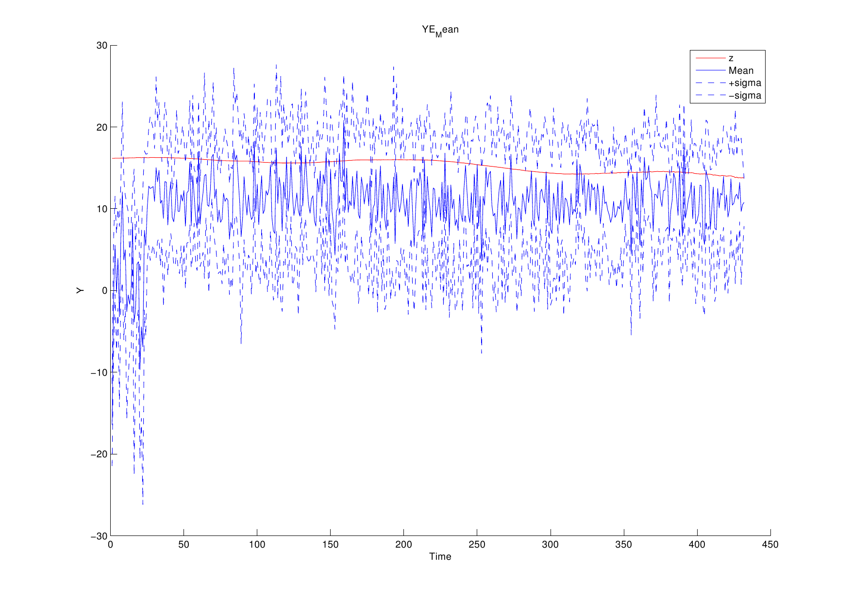
PMCMC marginal likelihood estimation of incremental marginal
likelihood sequence for each dimension of the observation
vectors for Lorenz model versus true incremental marginal
likelihood.
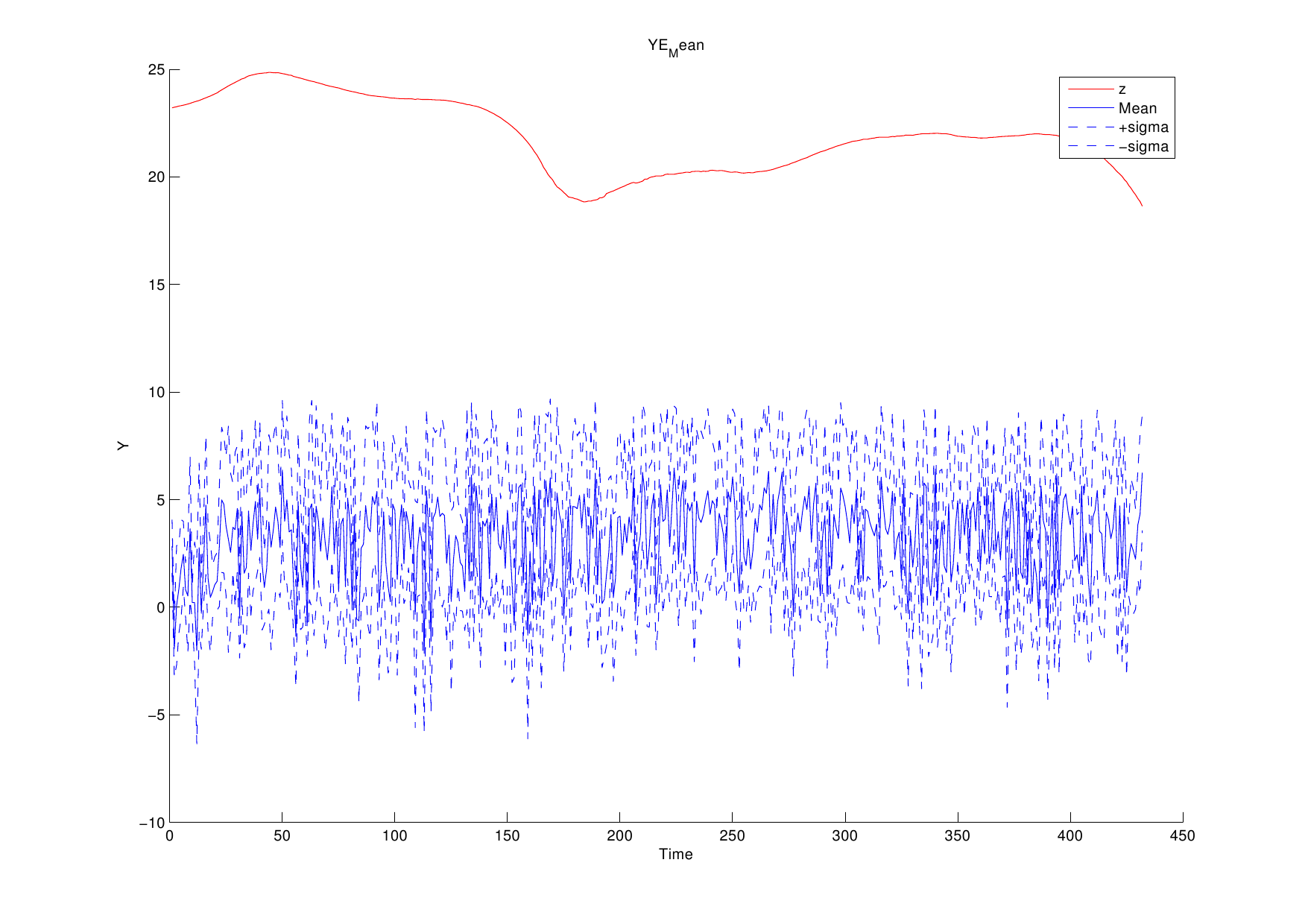
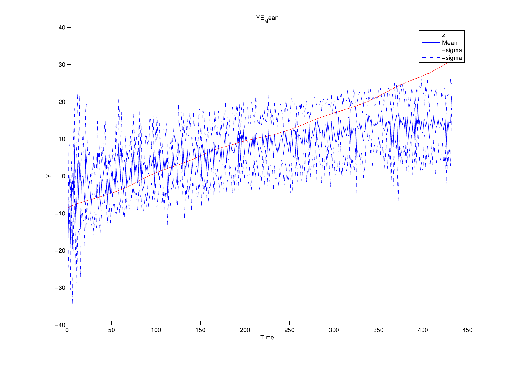
The average of mean functions from
the estimated model at each MCMC iteration (y1, y2,
y3 in turn)
The above figures could be obtained by using the following function of this toolbox,
Graphs.YEMean(PathForOutput, PathForMatFile);
where PathForOutput is the filename path for these figures to be saved and
PathForMatFile is the matlab filename which contains the estimated parameters.
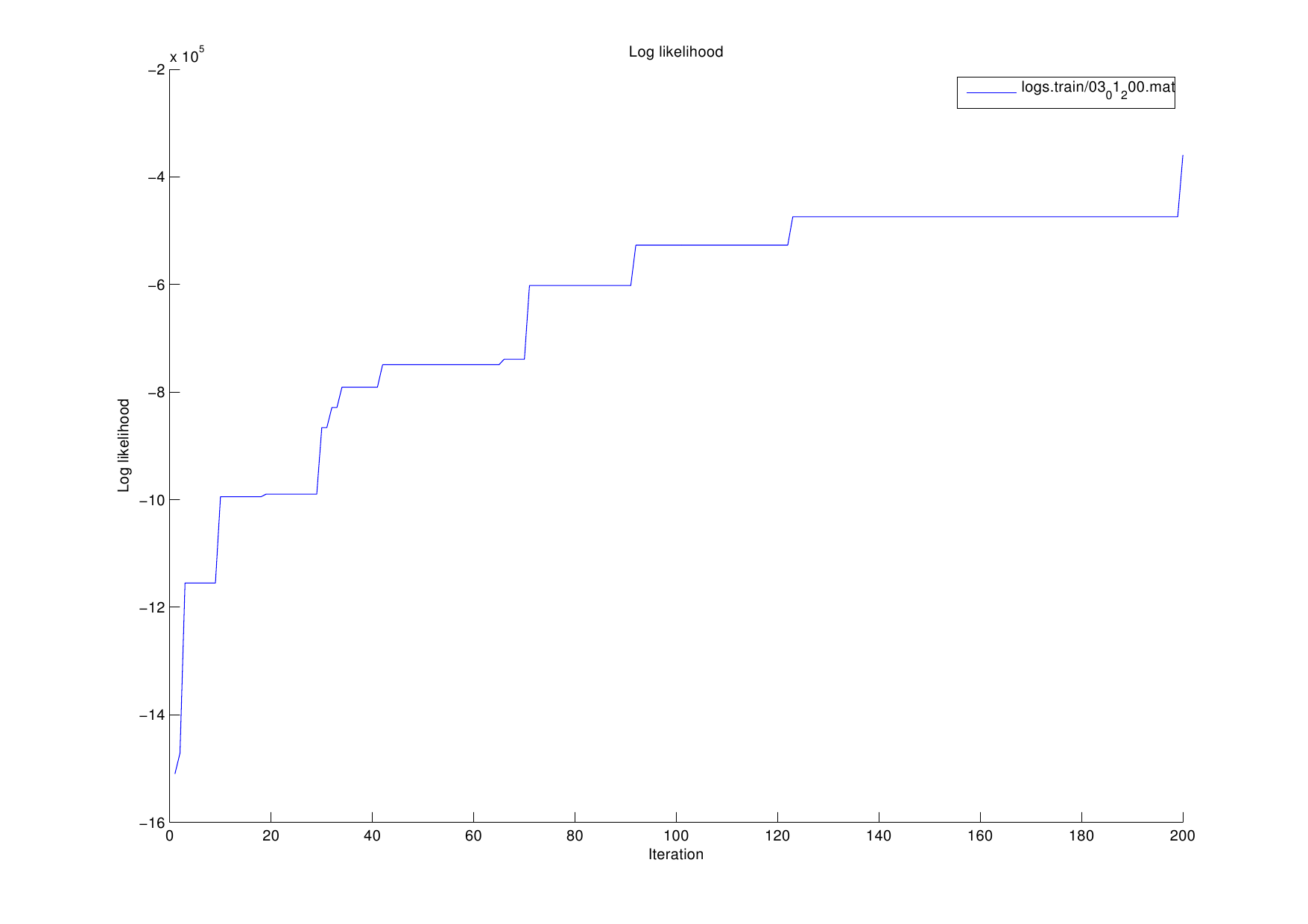
The log-likelihood estimated at each
MCMC iteration
The above figure could be obtained by using the following function of this toolbox,
where PathForOutput is the filename path for this figure to be saved.
Having trained this model, we can now assess the MCDC Test
function using the trained models on each of the left out
experimental videos in the leave-one-out cross validation.
When considering these results we observe that we expect that
the trained model, based on an a prior belief that a linear
constant velocity structure is present, should not be optimal
for several movements which are more complex with different
angular accelerations and non-straight line trajectories.
Hence, the trained GP-SSM from subjects 7 and 9 are expected
to work more appropriately than the other motions.
In this experiment, we first estimated the parameters of
GP-SSMs for each trial data using the PMCMC2 method and created
each model. Each trial data/model is assigned to the subject.
Then, we examined to classify each trial data to the subject
of the model which shows the highest marginal likelihood
between all models except for the model of the data examined.
It is shown that the MCDCTest function reasonably performs
especially for subjects 7 and 9. While the motions of subjects
7 and 9 are relatively stable, the motions of subjects 3 and 5
are dynamically changeable and consequently less likely to be
adequately explained by the a prior belief of a linear
Gaussian dynamic structure. Improvements in these
classifications can be made with non-constant velocity mean
functions and non-homogeneous assumptions of the GP covariance
kernel.
Source code: samples/MotionCapturePMCMC2Test.m
Commands:
addpath('samples');
MotionCapturePMCMC2test;
| Subject # |
Estimated subject number
|
| 3 |
5 |
7 |
9 |
Target subject number
|
3 |
1 |
2 |
1 |
0 |
| 5 |
0 |
5 |
3 |
12 |
| 7 |
0 |
1 |
7 |
4 |
| 9 |
0 |
1 |
0 |
11 |
Classification accuracy in the model classification
experiment
| Subject # |
Session Description |
# of correctly classified trials
|
Total
|
Accuracy
|
| 3 |
walk on uneven terrain |
1 |
4 |
25.0% |
| 5 |
modern dance |
5 |
20 |
25.0% |
| 7 |
walk |
7 |
12 |
58.3% |
| 9 |
run |
11 |
12 |
91.7% |
| 合計 |
24 |
48 |
50.0% |